
Corrective Model
In its maximum resolution configuration, HARMONI will be able to resolve objects as small as 10 milliarcseconds wide. This does not only determine the performance figures of the optics directly involved in the observation, but also the accuracy requirements of the pointing of the telescope.
Unfortunately, it is unfeasible to command ELT to point towards a given sky coordinate and expect it to stay there for the duration of the observation. ELT is too big for that, and external effects like wind, thermal expansion or its own weight will move the instrument’s field center from its intended location.
As with other telescopes of its kind, pointing is automatic, and operates in closed loop mode. This means that HARMONI will need to find a pointing reference first (up to 2 known guide stars) and compare its location with respect to the location it should be in if the pointing was correct. The result of this comparison takes the form of an angular distance, and represents an immediate measurement of the pointing error. This process is performed in a continuous loop, delivering the measurements back to ELT, so that it can correct its pointing in real time.
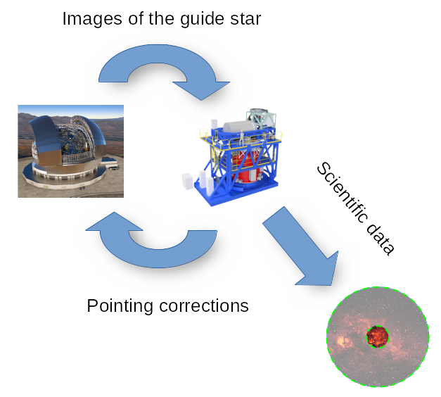
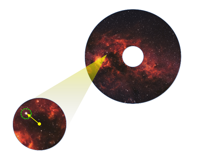
Pointing error measurements are not performed directly in the telescope’s focal plane, but in a relayed focal plane inside the instrument with unitary magnification. This relayed focal plane is physically located inside LOWFS, in a controlled temperature environment. In order to perform a measurement of the pointing error, LOWFS features two robotic arms (the pick-off arms, POA for short) with a tilted mirror on their ends. These robotic arms will place their mirrors in the image of the guide stars, forwarding their light to the detector used for measurement. Although the POAs can be placed anywhere in the relayed focal plane, pointing measurements are restricted to an annular region named the technical field. This ensures that the central circular region (named the science field) is never blocked by the POAs, making it suitable for science observations.
Correcting the instrumental signature
It is reasonable to think that the measurements of the pointing error need to be at least as accurate as the target pointing accuracy. However, manufacturing tolerances and slow-varying effects may introduce systematic biases in the measurements, preventing us from reaching the desired accuracy. A non-comprehensive list of the potential sources of bias could be:
- Relay optics distortion
- POA encoder errors
- Derotator wobbling
- Thermal expansion
- Other slow-varying effects (structure deformations?)
All of these biases are encompassed under the concept of the instrumental signature, referring to any pointing error caused by the instrument alone, and whose effects must be corrected. This correction is done by the corrective model, which is nothing but a transformation between coordinates of the telescope’s focal plane and coordinates of the relayed focal plane.
Of course, these biases are initially unknown and must be calibrated before performing any observation. Calibrations will be carried out by means of the Geometrical Calibration Unit (GCU). The GCU features a retractable mask consisting of a fixed pattern of point light sources with known locations. This mask can be physically inserted in the telescope’s focal plane, enabling HARMONI to observe its own distortions. The difference between the observed locations with respect to their nominal locations are used as input data to the calibration procedure, which fits the corrective model to the observed distortion.
The formulation of the corrective model
The current proposal for the corrective model takes the form of a truncated expansion of complex Zernike polynomials (also called pseudo-Zernike polynomials). These polynomials can be seen as orthogonal basis vectors of continuous 2-D vector fields defined on the unit circle. The complex formulation allows us to identify the real and imaginary parts of the complex quantities with the horizontal and vertical projections of 2-D vectors in the focal plane, simplifying the mathematics needed to describe the distortion.
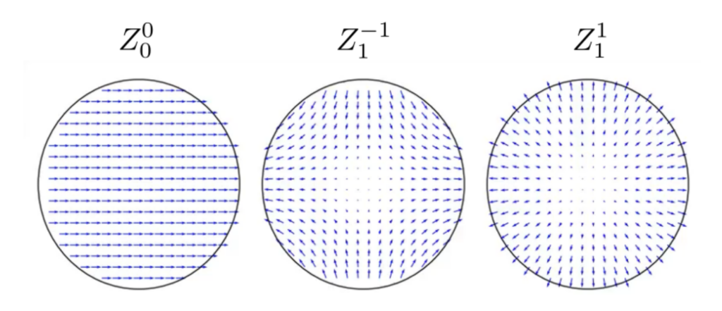
The expansion will be used to model the displacement vector \(\vec{\varepsilon}(\vec x)\) of the observed calibration points with respect to their nominal positions, and will be used by the observatory both to command the POAs and interpret the results of the measurements:
$$
\vec{\varepsilon}(\vec x) \approx \sum_{j=0}^{J-1} \hat{\alpha}^j\hat{Z}_j\left(\frac{\vec x}{R}\right)
$$
With \(R\) the radius of the focal plane, \(J\) the number of polynomials in the expansion (assuming OSA/ANSI indices), \(\hat{Z}_j\) the complex Zernike polynomial representing the \(j\)-th basis distortion and \(\hat{\alpha}^j\) a complex number encoding the magnitude and angle of the \(j\)-th basis distortion. We call these \(\hat{\alpha}^j\) the model coefficients.
The interest of this expansion lies in which each polynomial can be connected to a distortion with physical interpretation. For instance, the first polynomial represents a global displacement of the points in the relayed focal plane. The next 2 represent changes in aspect ratio and a rotation / scale change, and so on.
Fitting the corrective model
Another interesting property of the current formulation of the corrective model is its linearity. This means that, given \(J\) or more measurements of the instrumental pointing error in \(J\) different points (\(\vec{\varepsilon}^j\)), all the \(\hat{\alpha}^j\) can be naively obtained by solving a linear system of equations with \(J\) unknowns.
Nonetheless, while this approach seems the most reasonable thing to do, is not free of limitations:
- In order to solve a system of equations with \(J\) unknowns, we need at least \(J\) equations (\(J\) calibration points). If \(J\) is large, this would imply an equally large number of commandings of the POAs, resulting in long calibration times.
- The POAs (along with their corresponding detectors) are measurement devices. This means they are affected by measurement noise, impairing the quality of the fit.
- Not all points provide the same amount of information about the distortion (e.g. a point in the middle may provide information about the global displacement of the mask, but not about its rotation).
- Not all combinations of points are equally valid. If two calibration points are too close together, the system matrix may be ill-conditioned, amplifying the effect of the measurement noise.
In order to address this limitations, we propose a Bayesian calibration technique. This technique exploits the fact that, while certain low-order distortions are expected to vary from one observation to the next, high-order distortions are caused by the relay optics and we expect them to have a much smaller variation.
Under this approach, we do not work with individual coefficients but with the joint probability distributions thereof, estimated from a finite set of previous (classical) calibrations. Each individual measurement of the instrument distortion (along with its nominal accuracy) updates the prior knowledge we have on them. The result of each update is a posterior joint distribution of the coefficients that can be used to derive a good representative of the model coefficients (i.e. the means) and calculate the degree of certainty we have on the residual of the model.
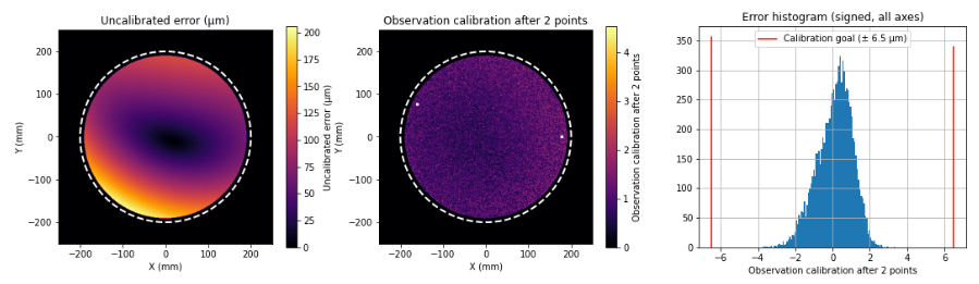
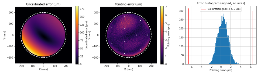
Pointing simulations of the instrument showed that, for distortions up to the 10 first Zernike moments, only 3 measurements were needed to calibrate the instrument up to the desired accuracy (and, in some cases, only 2) with an almost flat residual along the field. On the other hand, classical calibration required at least 10 carefully-chosen calibration points with visible spatial structure on the residual of the model.